Computer vision has been a great success of deep machine learning. It is now widely used in many practical applications such as object recognition, classification and detection, self-driving cars, image captioning, image reconstruction, and generation. We present a primer on computer vision starting with how we understand vision in humans.
Vision Recognition
Human eye
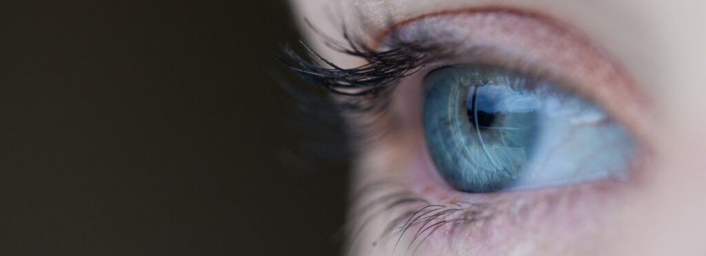
Vision recognition with a human works by capturing light refracted through the cornea, the anterior chamber, the pupil, the posterior chamber, the lens, the vitreous humor, and then the retina in the back of the eye (Figure 1). The pupil adjusts the aperture of the eye letting more or less light in depending on the need to focus or the ambient light.
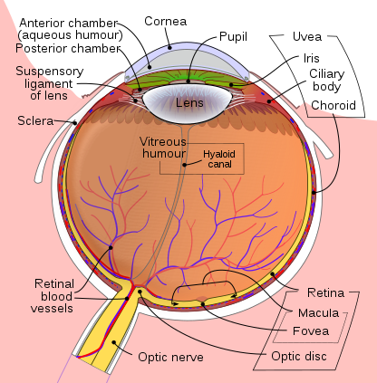
Figure 1. Eye. Rhcastilhos. And Jmarchn., CC BY-SA 3.0 <https://creativecommons.org/licenses/by-sa/3.0>, via Wikimedia Commons
The retina contains photoreceptor cells made of rods (sensitive to light) and cones (sensitive to color), bipolar cells, and ganglion cells (Figure 2). All these cells are neurons. The ganglion cells then form the optic nerve with their axons. Through the rods and cones, the photons generate electrical signals by phototransduction.
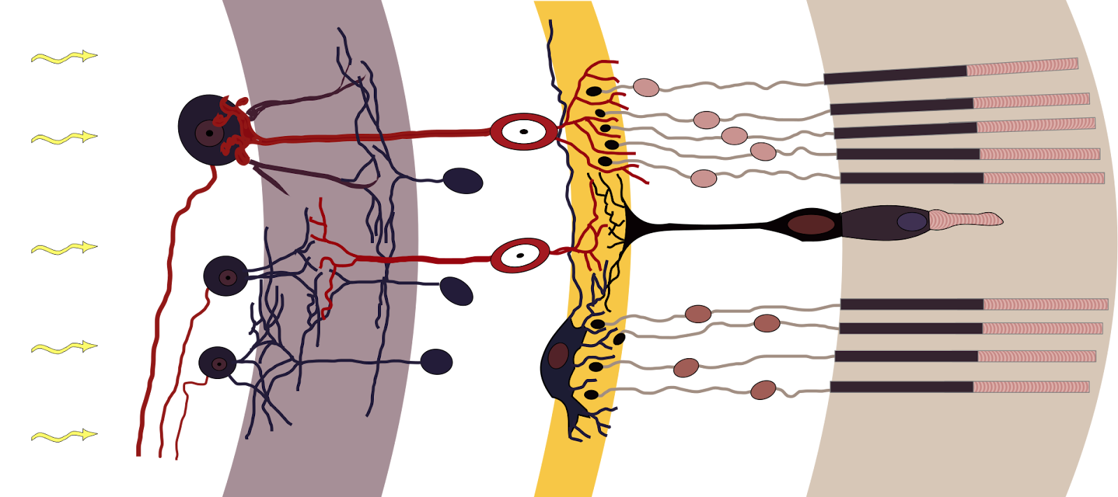
Figure 2. Retinal layers. By Fig_retine.png: Ramón y Cajalderivative work Fig retine bended.png: Anka Friedrich (talk)derivative work: vectorisation by chris 論 – Fig_retine.pngFig retine bended.png, CC BY-SA 3.0, https://commons.wikimedia.org/w/index.php?curid=7550631
The optic nerve then connects to the optic tract and to the Lateral geniculate nuclei (LNG, left and right) situated in the thalamus and then, in turn, connect to the Primary visual cortex through the optic radiations (Figure 3). The visual information is processed in the Primary visual cortex (also called the visual area V1).
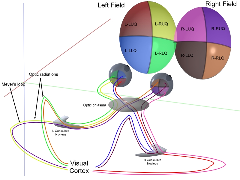
Figure 3. Optical cabling. Ratznium at en.wikipedia, CC BY-SA 3.0 <http://creativecommons.org/licenses/by-sa/3.0/>, via Wikimedia Commons
Hubel and Wiesel experiment
In 1958, Two scientists at Johns Hopkins University who later received the Nobel Prize in Medicine, David Hubel and Torsten Wiesel discovered that neurons in the striate cortex, part of the visual cortex, were activated by particular oriented lines and movements. They used kittens looking at a projector screen with tungsten microelectrodes inserted in the visual cortex connected to an oscilloscope to measure neuron activation. They initially investigated the neuron cell activation with black dots on a white slide till they accidentally showed the edge of the slide which triggered the neuron to fire. They found that field receptors on the neuron were being activated by specific oriented patterns (slit, dark bar, or edge) and movements. Some receptors were either excited or inhibited and have a particular geometry that matches the specific pattern they are reacting to. Neuron cells reacting to the same pattern are organized in vertical columns and neighboring cells are reacting to patterns of similar shape but slightly of different orientation.
Figure 4. Field receptors on a simple neuron cell are aligned with the pattern they react to
Convolutional Networks
Convolutional networks are inspired by the visual processing described in the previous section. Convolutional networks are particular cases of deep learning networks with layers of convolutions applied to images.
Convolution
Convolution is a mathematical operation that mixes two functions by multiplying their values by pairs. One version of convolution used in machine learning consists of multiplying pairs of values evaluated at the same point. This is called the cross-correlation.
One function works as the signal, the second function works as a filter. Figure 5 gives some examples of convolutional filters. The input signal is a 5×5 matrix with numerical values. It could be some color or light intensity. The input signal goes through the filter by multiplying each input cell by the corresponding filter cell in the same position. The input signal is then transformed into a filtered signal (also called the feature map). The output is calculated as the sum of all the values in the filtered signal.
The filters can be of different types. Each filter represents a different channel. Filter A at the top detects diagonal signals by filtering only values close to the main diagonal. Filter B detects horizontal signals and filter C detects signals on the secondary diagonal. If there is no overlap between the input signal and the filter, the final output value is zero. If the overlap is very large then the final output value is very large.
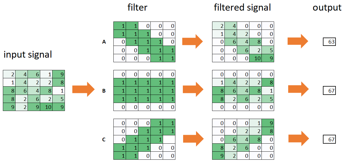
Figure 5. Examples of convolutional filters
The filters can amplify the input signal or even invert it (by using negative values). Like the neurons in the visual cortex, each filter is specialized in detecting special features.
An image is however larger and more complex than a 5×5 matrix. A solution is to use different filters and make them scan the image starting from left to right then top to bottom. This is illustrated in Figure 6 (with a 10×10 image and a 3×3 filter). The convolution operation starts with the top-left submatrix and continues to the subsequent matrices on the right by moving by one column (the stride which can be 1 or a higher value) till all the cells are covered and then towards the bottom by moving by one row (or more). The output ends up being an 8×8 matrix. To maintain the 10×10 size it is possible to add paddings of 0 values by adding extra rows and columns around the initial input image.
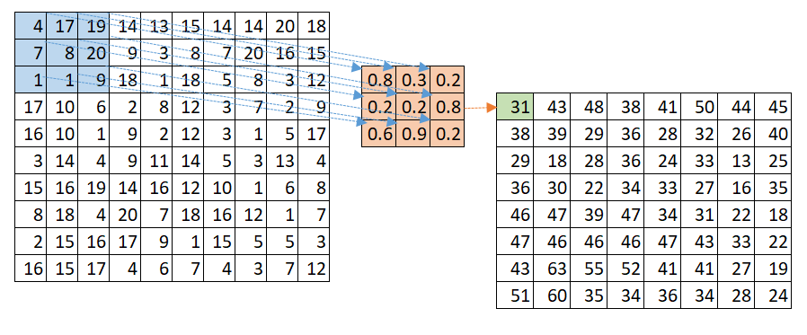
Figure 6. Convolutional Neural Network with a (3,3) Convolution
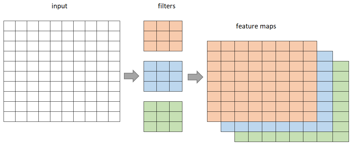
Figure 7. Convolutional Neural Network with 3 channels
Max pooling and average pooling
Besides convolution, another common operation is max pooling (Figure 8) and average pooling (Figure 9). With max pooling, the filter selects the maximum value of the matrix cells it is covering instead of multiplying the cells with some weights and summing the results. With average pooling, the filter calculates the average values of the matrix cells. Average pooling is a particular case of convolution where the weights in the filter have the same value and are normalized to sum up to one.
The pooling layers perform these pooling operations which aggregate the signals and downsize the image files (also called downsampling). Some information is lost during pooling operations. Some more recent techniques avoid pooling for that reason.

Figure 8. Convolutional Neural Network with Max Pooling
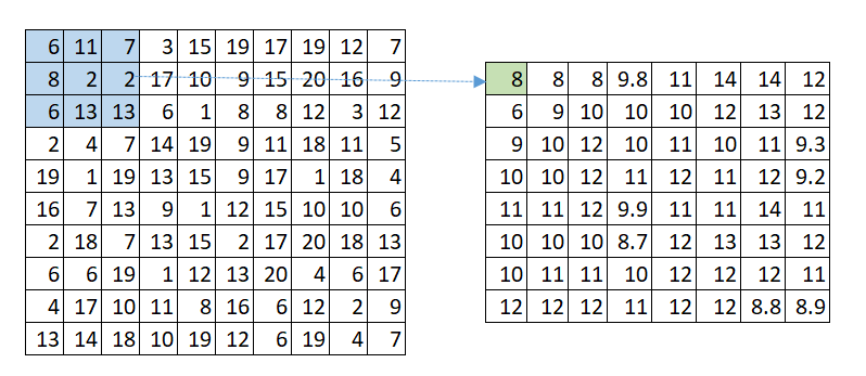
Figure 9. Convolutional Neural Network with Average Pooling
Translation equivariance
Convolutional networks have the property that they perform equally well at identifying and classifying an object if it moves horizontally or vertically in the image. The reason is that the same filters are also translated in the image. This is called translation equivariance. Convolutional networks are however not indifferent to rotation or inversion. They probably would be if filters were to rotate and be inverted. A solution is data augmentation. Images can be rotated and inverted and added to the training data.
Locality
Convolutional networks operate at the local level. They identify features in limited parts of the image as defined by the filter size and feed the features through several layers of neural networks.
Benchmarks
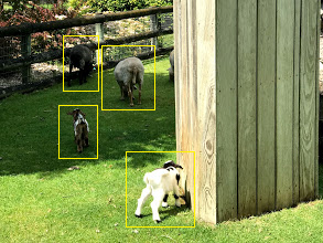
Figure 9. Image localization and identification
ImageNet
ImageNet is an image database created in 2009 by Professor Fei-Fei Li and her team as a benchmark for visual recognition and classification tasks. It contains over 14 million images from the internet annotated by humans around 20,000 categories called Synonym Sets (synsets). A higher-order category could be “fish” and be divided into hundreds of synsets of fish species that have hundreds of images of fish each. ImageNet is used for the ImageNet Large Scale Visual Recognition Challenge, started in 2010, in which researchers compete to detect and classify objects in images and videos. AlexNet (Krizhevsky et al., 2017) won the competition in 2012 using convolutional neural networks. The competition has been hosted by Kaggle since 2017. Its validation and test sets have 150,000 photographs and 1,000 categories. The training set is randomly sampled from these sets. Each photograph in the training and validation set has the coordinates of bounding boxes with the attached object category.
MNIST
MNIST is a dataset on handwritten digits that has been used by LeCun (1988) for visual recognition. It has 60,000 digits in the training set and 10,000 in the test set. Each digit occupies a 28×28 grid. 250 human writers, a mix of Census employees and high school students, created these digits in the training set and another 250 did the same for the test set.
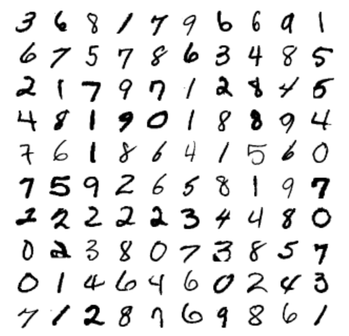
Figure 10. Examples of MNIST digits. Source LeCun et a;. 1998
Fashion MNIST
Fashion MNIST has the same structure as MNIST but is based on clothing articles from the company Zalando. Like MNIST, it has 60,000 images in the training set and 10,000 images in the test set. The size of each image is also 28×28. It also has ten categories ( 0: T-shirt/top, 1: Trouser, 2: Pullover, 3: Dress, 4: Coat, 5: Sandal, 6: Shirt, 7: Sneaker, 8: Bag, 9: Ankle boot). The difference is that the task is more difficult because the clothing articles have more variations than written digits.
Figure 11. Clothing articles from Fashion MNIST. Source: https://github.com/zalandoresearch/fashion-mnist/blob/master/doc/img/fashion-mnist-sprite.png
CIFAR-10 and CIFAR-100
CIFAR-10 is a dataset with 60,000 photos classified in 10 categories. CIFAR-100 is an extension of CIFAR-10 with 100 categories.
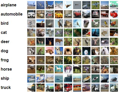
Figure 12. Photos from CIFAR-10. Source: https://www.cs.toronto.edu/~kriz/cifar.html
Convolutional Network Models
AlexNet
Building on convolution networks such as LeNet by (LeCun et al., 1989) (Figure 13), (Krizhevsky et al., 2012) proposed AlexNet in 2012 that won the ImageNet competition and put deep learning networks on the map for computer vision. They successfully classify 1.2 images into 1,000 classes with state-of-the-art results at the time.
AlexNet uses five convolutional layers, max-pooling layers, and three fully-connected layers (Figure 14) and ReLU activation functions. Images are of size 224×224 with three channels (RGB colors). To prevent overfitting, it performs data augmentation by extracting 224×224 patches and their inverses (horizontal reflections) from 256×256 images and by changing the RGB channel intensities. They also use dropout to reduce overfitting.
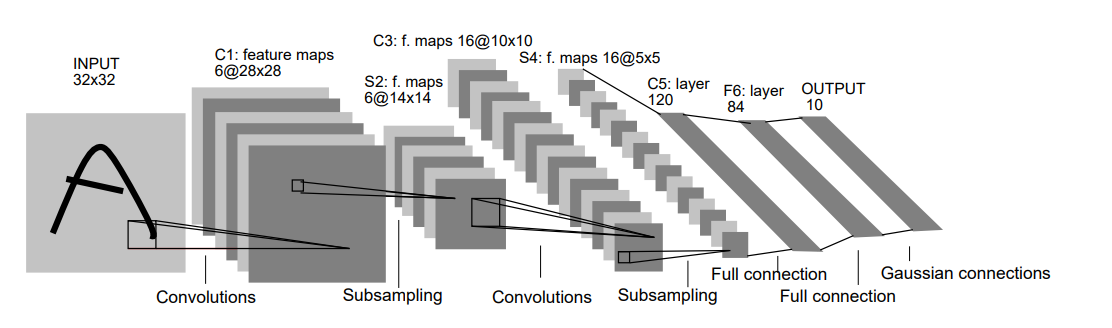
Figure 13. LeNet architecture
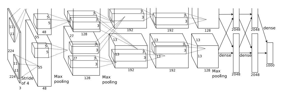
Figure 14. AlexNet architecture
GoogleNet
GoogleNet is based on the inception network as described in(Szegedy et al., 2014). A basic building block is the inception module. The inception modules were inspired by the Network in Network of (Lin et al., 2014). They allow a shift from sparse to dense representations using smaller filter-size convolutions (1×1, 3×3, 5×5), enhance the representativeness of the network and perform dimensionality reduction. The whole network will be built by stacking inceptions modules. These modules are stacked 22 times in GoogleNet.
In their inception module (Figure 15), a layer goes through three 1×1 convolutions and a 3×3 max pooling, then 3×3 convolutions, 5×5 convolutions and 1×1 convolutions. Outputs are then concatenated. The whole network is presented in Figure 16. GoogleNet achieves very good results in the ImageNet Large Scale Visual Recognition Challenge (ILSVRC) 2014 Classification (first) and Detection (second) Challenges.
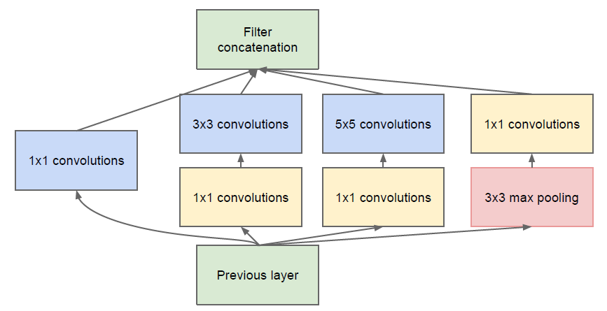
Figure 15. Inception module. Source: Szegedy et al., 2014
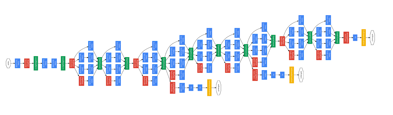
Figure 16. GoogleNet
VGG
VGGNet was introduced in (Simonyan and Zisserman, 2015) as an extension of standard convolutional networks such as LeNet and AlexNet with the difference that the network is deeper with 16-19 layers and with smaller (3×3) convolutional filters. They achieved 2nd and 1st place in the 2014 ImageNet Challenge in classification and localization. The increase in depth and the smaller receptive fields of the convolutions reduce the number of parameters compared to a standard convolutional network and work as a regularizer of the network. The configuration for VGG-16 (16 weight layers) combines stacked of two 3×3 convolutions with 64, 128, 256, 512, and 512 channels respectively, max-pooling layers and full and three fully connected layers of size 4096, 4096, and 1000 (for the 1000 classes). The activation function is ReLU. Figure 17 shows a truncated VGG-19 network.
ResNet
Residual networks (ResNet) introduced by (He et al., 2015b) are networks similar to VGG networks but with skip connections. These skip connections (Figure 17, the loops are the skip connections in the 34-Layer ResNet) connect inputs to outputs by adding the input values to the layer outputs coming from convolutional networks. Because the identity function is forced into the output at each step, the model focuses on fitting the residuals from the identity, a task that is easier to achieve as the authors have documented. Models can be very deep without encountering optimization problems or vanishing/exploding gradient issues. They evaluate their model on ImageNet and on CIFAR-10. Their ResNet model with 152 layers won the ILSVRC in 2015.
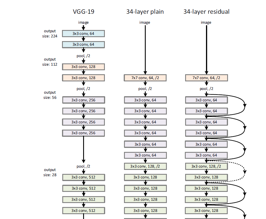
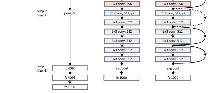
Figure 17. VGG Net vs 34-Layer plain and 34-Layer ResNet. Source: (He et al., 2015b)
References
Goodfellow, I., Bengio, Y., Courville, A., 2016. Deep Learning, Illustrated edition. ed. The MIT Press, Cambridge, Massachusetts.
He, K., Zhang, X., Ren, S., Sun, J., 2015a. Delving Deep into Rectifiers: Surpassing Human-Level Performance on ImageNet Classification. ArXiv150201852 Cs.
He, K., Zhang, X., Ren, S., Sun, J., 2015b. Deep Residual Learning for Image Recognition. ArXiv151203385 Cs.
Krizhevsky, A., Sutskever, I., Hinton, G.E., 2012. ImageNet Classification with Deep Convolutional Neural Networks. Adv. Neural Inf. Process. Syst. 25, 1097–1105.
LeCun, Y., Boser, B., Denker, J.S., Henderson, D., Howard, R.E., Hubbard, W., Jackel, L.D., 1989. Backpropagation applied to handwritten zip code recognition. Neural Comput. 1, 541–551. https://doi.org/10.1162/neco.1989.1.4.541
Lin, M., Chen, Q., Yan, S., 2014. Network In Network. ArXiv13124400 Cs.
Simonyan, K., Zisserman, A., 2015. Very Deep Convolutional Networks for Large-Scale Image Recognition. ArXiv14091556 Cs.
Srivastava, N., Hinton, G., Krizhevsky, A., Sutskever, I., Salakhutdinov, R., 2014. Dropout: A Simple Way to Prevent Neural Networks from Overfitting. J. Mach. Learn. Res. 15, 1929–1958.
Szegedy, C., Liu, W., Jia, Y., Sermanet, P., Reed, S., Anguelov, D., Erhan, D., Vanhoucke, V., Rabinovich, A., 2014. Going Deeper with Convolutions. ArXiv14094842 Cs.