
A Primer on Natural Language Processing
The Field of Natural Language Processing
Natural Language Processing is one of the fastest evolving fields in AI and machine learning. It might also be the shortest path to understand intelligence. When we think of an intelligent machine, we imagine a machine that can communicate with us, that has language skills.
Alan Turing in his famous 1950 paper on Computing Machinery and Intelligence (“I.—COMPUTING MACHINERY AND INTELLIGENCE | Mind | Oxford Academic,” 1950) proposes to answer the question “Can Machine Thinks?” with an Imitation Game (now called the Turing test) based on language. A machine that can have a natural conversation with a human would be considered a thinking machine. Solving AI would therefore be equivalent to solving NLP.
Solving NLP involves many practical tasks that should be useful beyond looking for artificial general intelligence. In this chapter, we review some of these tasks and go over the different models which are used in modern deep learning NLP including the GPT-3 model.
Language Tasks
NLP tasks are as diverse as the different uses of natural language. We present a non-exhaustive list of tasks: Question answering, machine translation, named entity extraction, coreference resolution, semantic role labeling, sentiment analysis, textual entailment.
Question answering
A question answering task tests reading comprehension of an NPL system. The NLP system should be able to answer questions. The prevalent benchmark is the Stanford Question Answering Dataset (SQuAD) (Rajpurkar et al., 2016). It contains a list of 100k questions with answers identified as a segment of text (a span) in a Wikipedia entry. For instance to the question “What causes precipitation to fall?”, it answers “gravity”.
The latest version, SQuaD, also includes 50k unanswerable questions. If the question does not have answers, a system should not offer one. An NPL system is given the question and has to retrieve the answer from the Wikipedia articles. It is evaluated according to its F1 score (F1 Score = 2*(Recall * Precision) / (Recall + Precision)).
Machine translation
Machine translation is one of the most popular applications of NLP and is used in tools such as Google Translate or on Facebook to translate posts. Datasets used for machine translation are provided by the Workshop on Statistical Machine Translation (WMT) (“Translation Task – ACL 2014 Ninth Workshop on Statistical Machine Translation,” n.d.). They include the WMT2014 English-German dataset and the WMT2014 English-French dataset.
The models are evaluated with the BLEU score which considers human translation as the benchmark. The Bilingual Evaluation Understudy (BLEU) (Papineni et al., 2002)) is a precision measure. It counts the matches of 4-grams to the human translation and makes adjustments for the length of the translation. The BLEU score is found to be highly correlated with the human judgment of translation quality.
Named entity extraction
Named entity extraction identifies named entities in a text and assigns them to different categories such as persons, organizations and locations, or miscellaneous entities. This task is useful to search, reference, or classify documents. It has to identify the named entities, which can be one or several tokens such as the United States of America, and then classify the named entity correctly. It is evaluated according to its F1 score. A benchmark database is the Reuters RCV1 corpus (“Reuters Corpora @ NIST,” n.d.)with annotated entity classifications.
Coreference resolution
Coreference resolution consists of linking worlds referring to the same entity, especially pronouns in a sentence. For instance, a benchmark database is the OntoNotes coreference annotations (“OntoNotes Release 5.0 – Linguistic Data Consortium,” n.d.). It is evaluated according to its F1 score. An example of coreference resolution is the Winograd Schema Challenge. In the sentence “The city councilmen refused the demonstrators a permit because they [feared/advocated] violence.” Depending on which verb is used, “they” refer to either the “city councilmen” (“feared”) or “demonstrators” (“advocated”). So some deep understanding of the sentence seems to be required to identify the correct coreference. The Winograd Schema Challenge has been compared to the Turing Test.
Semantic role labeling
Semantic role labeling consists of labeling words according to their role around a predicate in a sentence. For instance, The Proposition Bank or PropBank (“The Proposition Bank (PropBank),” n.d.), built on top of the Penn Treebank (“Treebank-3 – Linguistic Data Consortium,” n.d.), has a list of annotated sentences with verb predicates and defined roles for each argument of the predicate. The roles are specific for each verb predicate. For the predicate “agree”, the roles are “Agreer”, ”Proposition”, and “Other entity agreeing”. Another common source of labeling is FrameNet which is focused on frames and frame elements instead of a verb predicate and OntoNotes which build on top of the Penn Treebank for syntax, and Propbank for predicate-argument structure.
Sentiment analysis
Sentiment analysis deals with the polarity, positive or negative, of a sentence or piece of text. It can be applied to movie reviews, product reviews, written reports, news articles, social media posts, or customer voice interactions. A standard database with annotated sentiments is the Stanford Sentiment Treebank (“Treebank-3 – Linguistic Data Consortium,” n.d.) which uses around 11,000 sentences from movie reviews. Each movie review falls into one of five categories from very negative, negative, somewhat negative, neutral to somewhat positive, positive, and very positive as classified by Amazon mechanical Turks. A Bag of word approach can be used where each word is given a sentiment score but is sometimes not sufficient because it lacks context and order.
Textual entailment
Textual entailment is the relationship between a text and a hypothesis. Given a text or fact, the NLP system has to evaluate if a hypothesis is True (entailment), False (contradiction), or Neutral. A benchmark is the Stanford Natural Language Inference (SNLI)(“The Stanford Natural Language Processing Group,” n.d.). It has 570k entries of text, judgments (entailment, contradiction, or neutral), and hypothesis. For instance, the text could be “A soccer game with multiple males playing.”, the hypothesis is “A soccer game with multiple males playing.” and the judgment is “entailment”, because the hypothesis is backed by the text. If the text is “A black race car starts up in front of a crowd of people.” and the hypothesis is “A man is driving down a lonely road.” then the judgment is “contradiction”.
Other tasks
There are many other tasks such as speech recognition (used by personal assistants such as Siri or Alexa), text-to-speech to read texts, text summarization to summarize news articles, reports, or books, text classification to screen for email spams, offensive contents, or identify authorship, information extraction to collect data from web pages or online documents, information retrieval to find relevant documents or pieces of information (used in search engines in Google, YouTube or Amazon).
Classical NLP Modelling
Symbolic NLP
To solve these tasks one approach is to teach the computer vocabulary, syntax, and grammar, the rules of language. This approach is symbolic NLP and uses parsing techniques to identify the words, their roles, and their meanings (Part-of-Speech or POS tagging). Because of the complexity and ambiguity of language and its relative free form, it is difficult to make a hand-written inventory of all the rules required to understand and generate language.
Another approach is to learn language probabilistically, using a statistical language model that is trained on real-world data. Because of the now extremely large amount of digital text available with corpora of millions, billions, and even trillions of words, and the large availability of computing power, the statistical approach has gained the upper ground while the symbolic approach has not made meaningful progress in real-world applications. MIT Professor Noam Chomsky has been very critical of the statistical approach despite of its success. He was quoted as saying:
“It’s true there’s been a lot of work on trying to apply statistical models to various linguistic problems. I think there have been some successes, but a lot of failures. There is a notion of success … which I think is novel in the history of science. It interprets success as approximating unanalyzed data.” (“Pinker/Chomsky Q&A from MIT150 Panel,” n.d.)
Norvig (“On Chomsky and the Two Cultures of Statistical Learning,” n.d.) has an interesting article addressing his criticism. In particular, he points out the empirical success of these models applied to search engines (Norvig works at Google), speech recognition, machine translation, and question answering.
Language Model
A language model describes the probability distribution of words. It is a statistical representation of language. It answers the question of what is the probability that a word appears after a sequence of words, or what is the probability that a sentence was said vs another one. This is a very powerful approach to develop language applications because it can leverage existing textual data and can tell for instance, if a sentence is grammatically correct or logical because correct and logical sentences are more likely to occur in the data.
Bag of words
The simplest language model is the bag-of-words model where only the frequency of each word matters, not the ordering nor the presence of other words. It is a poor model to generate sentences but it is useful to measure sentiment or classify text. If some words tend to appear more frequently in a negative sentence, their presence can indicate that a sentence is likely to be negative, using the Bayes formula of conditional probabilities.
N-gram models
A more advanced approach than the bag-of-words is the N-gram model. In the N-gram model, the probability of each word is conditional on the previous N-1 words. A bigram model accounts only for the previous word, a 3-gram model will account for the previous two words, etc… Given these conditional probabilities, the probability of a full sentence can be calculated thanks to the law of iterated expectations. It will be expressed as a simple product of conditional probabilities or as the sum of logarithmic probabilities if logs are used. N-gram models can be used for spam detection, sentiment analysis, or document classification.
Deep NLP Modelling
Word Embedding and Word Vectors
The previous language models do not compare words. Two similar words or related words should be close in some dimension and word vectors allow these comparisons. Word vectors are also called world embeddings. Two successful approaches have been Glove and Word2Vec.
Glove (Global vectors)
Glove (Pennington et al., 2014) was developed at Stanford to construct vector representations of words. It is based on the co-occurences of words. Co-occurence means that words occur together in the same sentence. An unsupervised machine learning model on a corpus to estimate the co-occurence of pairs of words. The word vectors are estimated so that the dot product of two word vectors is equal to the probability of co-occurence. Thanks to this vector representation, relationships between words can be seen such as man to woman and king to queen.
Word2Vec
Word2Vec (Mikolov et al., 2013) was developed at Google and also aims to create word vectors where similar words have close representations. Closeness is measured either with the continuous bag of words (CBOW) or the continuous skip-gram. IWith continuous bag of words, a word is predicted according to its context. With continuous skip-gram a word predicts the context worlds surrounding it. A two layer neural network is used to estimate each model.
GLUE Benchmark
The General Language Understanding Evaluation (GLUE, (Wang et al., 2019)) benchmark is a set of tests to evaluate NLP models on different tasks of sentence understanding. Some tasks are based on individual sentences, some others on pairs of sentences.

Table 1. The GLUE tasks.
Because the new generations of NPL models tend to have superhuman performance in some tasks from the GLUE benchmark, SuperGLUE (Wang et al., 2020) has been introduced with more difficult and more varied tasks which also include human benchmarks.
Recurrent Neural Network (RNN)
RNNs (Elman, 1990) are a type of neural network that allows efficient modeling of sequences, such as time series or text data.
In a basic RNN, for each step t, an input vector x(t) is combined with a hidden vector or layer h(t-1) to produce an updated vector h(t) which then generates the vector y(t). In the next step t+1, the new input vector x(t+1) is combined with h(t) from the previous step to produce the new output vector y(t+1). The relationship between x(t+n),h(t+n-1),h(t+n),and x(t+n) is independent of n which makes it more efficient with fewer parameters to estimate.

Figure 1. Recurrent Neural Networks
The hidden layer h(t+n) keeps the memory of the previous step layers h(t+n-1),h(t+n-2),…,h(0). The parameters are estimated by back-propagation through time starting from the last period and moving back to the initial values of each layer.
As for a neural network with too many layers, the RNN can suffer from vanishing gradients t=(gradient becoming smaller and smaller as we go back in time) or exploding gradients (gradient becoming larger and larger). To address this issue, the LSTM model has been created.
Long Short Term Memory (LSTM)
LSTM was introduced in Hochreiter and Schmidhuber (Hochreiter and Schmidhuber, 1997). The LSTM uses a carry or memory cell c(t) which depends on an input gate it, and a forget gate f(t). The output depends on an output gate o(t).
The memory cell carries information from one step to the other but is more flexible than the hidden state. The information is copied with some adjustments. The memory cell depends on:
- input gate it: the input gate modulates the information from the input layer x(t) and the hidden layer h(t)
- a forget gate f(t): the forget date can erase some past memory cell information
The memory cell can therefore forget some past memory with the forget gate and use some new memory content thanks to the input fate. is the sigmoid function.
c(t+1)=f(t) ⊙ c(t)+i(t)⊙σ(b+Ux(t)+Wh(t))
⊙ is the element-wise multiplication.
The output uses an output gate o(t), the output gate modulates the memory cell c(t) to transform it into an output vector y(t). The output is calculated as:
yt=o(t)⊙tanh(ct)
The input gate, the output gate, and the forget date are updated with a sigmoid function :
i(t)=σ(b(i)+U(i)x(t)+W(i)h(t-1))
o(t)=σ(b(o)+U(o)x(t)+W(o)h(t-1))
f(t)=σ(b(f)+U(f)x(t)+W(f)h(t-1))

Figure 2. LTSM
The output y(t) will depend on the hidden state h(t) and memory cell c(t).
Compared to the simple RNN, the input layer x(t) does not feed the hidden layer h(t) directly but indirectly through the memory cell c(t). The hidden layer h(t-1) does not feed into the next hidden layer h(t) directly but only indirectly through the memory cell c(t).
Bi-directional LSTM
With the bidirectional LSTM (Graves and Schmidhuber, 2005), the same sequence is analyzed in reverse and the two LSTM outputs are combined by concatenation, sum, or product (Figure 3).

Figure 3. Bidirectional LSTM
Gated Recurrent Units (GRU)
The GRU was introduced by Cho (Cho et al., 2014) to simplify the LSTM. There is no more hidden layer. The output layer depends on an update gate u(t) and a reset gate r(t).
The update gate u(t) and the reset gate r(t) are updated with a sigmoid function :
u(t)=σ(b(u)+U(u)x(t)+W(u)y(t))
r(t)=σ(b(r)+U(r)x(t)+W(r)y(t))
The output layer y(t) is then updated as:
y(t+1)=u(t)⊙y(t)+(1-u(t))⊙(b+Ux(t)+Wr(t)⊙y(t))
Updating and resetting to a new value is determined in a single equation and bypasses a memory cell and a hidden layer.
ELMo (Embeddings from Language Models)
In traditional word embedding, a word can have only one meaning. ELmo, proposed in 2018 by the Allen AI Institute and the University of Washington (Peters et al., 2018), improves on traditional static word embeddings such as GloVe buy using the context of the word usage. It constructs vector representation of words based on the parameters of bidirectional on a LTSM model trained on a large text corpus. The representation depends on the whole sentence in which the world appears. These are contextualized representations since they depend on the context of the word.
The parameters are from all the layers of the biLSTMs and not only from the last layer.The parameters from the upper layers help understand context, while the parameters from the lower layers help to understand the syntax.
ELMo can be integrated to improve NLP tasks. The BLSTM model is run on the text and the ELMo representations and the status word representations are both fed into the supervised NLP tasks. ELMo improves the performance of many tasks such as question answering, text entailment, semantic role labeling, or coreference resolution.
Attention Model
Attention
The concept of attention allows to associate dynamically each word or token in a sequence to some words or tokens in another or the same sequence. This allows richer associations that do not depend on specific locations of the target words, in particular it can relate a word to words which are not in close proximity. This is useful in translation for instance where a meaningful word can be at the beginning of a sentence and still be useful to translate a word appearing at the end.
Attention (Vaswani et al., 2017) uses the concept of Queries, Keys, and Values. A Query is what we are looking for, the Key gives the location of what we are looking for and the Value is the result of the query. A Query is for instance a word, the key is a page in a dictionary where the word appears and the value is the translation of the word.
A word represented as an embedding vector x, is multiplied (matrix dot product) with a query weight matrix W(Q) to produce Queries Q, with a key weight matrix W(K) to produce Keys K. These matrices Q,K,V are then combined together and transformed into probabilities (through a softmax function and after normalization) to emphasize attention to specific values or tokens in the same sequence. The values V are calculated as the dot product between the initial token and a value weight matrix W(V).
The self-attention vector is then:
attention(Q,K,V)=softmax(QKᵀ/√d(k))V
d(k) is the dimension of the key vectors and is its square root is a normalization factor.
We can represent it in a picture:

Figure 4. Attention mechanism
attention(Q,K,V)is called a dot product attention (here a scaled dot product attention because of the scale factor). It would be called self-attention if the target sequence is the same. It is causal attention if attention cannot look forward and a mask is used to eliminate any forward looking attention. It is bimodal attention if attention can look backward and forward (two directions).
To have causal attention we just add to QKᵀ a triangular matrix M with 0 everywhere and -∞ in the upper triangular area of the matrix.
Multi-Head Attention
The procedure can me repeated several times with different W(Q,i),W(K,i),W(V,i) matrices to create several self-attention vectors or a “multi-head” attention. These vectors are then concatenated and multiplied by another weight matrix W(O) to produce a single self-attention vector.
z(i)=attention(Q(i),K(i),V(i)) for i=1,..,h if there are h heads.
Then
Multihead(Q,K,V)=Concat(z(1),…,z(h))W(O)
Transformers
Transformers (Vaswani et al., 2017) use the multi-head attention and as well as add & normalize layers, and feed-forward layers. A Transformer layer can combine an encoder and a decoder or use one only an encoder (as in BERT models) or only a decoder (as in GPT models).
They use as inputs word embeddings. Word embeddings are vector representations of words. Each word is represented by a vector of fixed dimension. The word embedding is a list of such vectors. The list size is fixed, usually equal to the longest sentence in a text.
Encoder
The encoder has four layers. As input it uses an embedding added to a positional encoding. The positional encoding indicates the location of each word vector. In the encoder, the input goes through a multi-head attention layer which encodes each word vector with other vectors which it needs to pay attention to. It is then added and normalized with the original layer input to preserve some memory of the input. It goes to a feed forward layer and again another add and normalize layer. The output is then fed into a multi-head attention layer of the decoder.

Figure 5. Transformer Encoder Layer
Decoder
The decoder is very similar to the encoder but it uses a masked multi-head attention layer to pay attention only to past word vectors.

Figure 6. Transformer Decoder Layer
Transformer
The Transformer layer uses a word embedding as input to the encoder, the result is fed into the decoder along with the output word embedding. The output word embedding is inputted into the first decoder layer repeatedly as new words get outputted.

Figure 7. Transformer
Transformers have launched a new wave of pre-trained language models such as BERT and GPT-3. We review some of them.
BERT (Bidirectional Encoder Representations from Transformers)
BERT is a pre-trained language model introduced by Google in 2018 (Devlin et al., 2019), that can be fine-tuned to perform many common NLP tasks such as the ones from the BLUE benchmark. Contrary to ELMo which uses the new embeddings as new features, BERT requires very little re-training.
BERT is using transformers with layers of decoders. It is trained first to identify randomly masked words (Masked Language Model) in a sentence using their contexts, words from the left and the right of the mask, and then to predict a next sentence (Next Sentence Prediction). It is therefore bidirectional contrary to GPT style models which are unidirectional. BERT uses a multi-layer bidirectional Transformer encoder.
There are two versions of BERT: BERT base and BERT large. BERT base has 12 layers of size 768, and 12 self-attention heads, and 110M parameters. BERT large has 24 layers of size 1024, and 16 self-attention heads, and 340M parameters. BERT is described in Figure 8.
BERT is pre-trained on a Corpus made of the BooksCorpus (800M words) and the English Wikipedia (2,500M words) representing a total of 3.3 billion words. The text goes through WordPiece tokenization and then runs through a masking step where tokens are masked at the rate of 15%. The token is replaced by [MASK] 80% of the time, by a random token 10% of time and remains the same 10% of the time. [MASK] is not used 100% of the time because it does appear in the fine-tuning step. BERT then goes through the Next Sentence Prediction step in which pairs of sentences can either be paired correctly with label [IsNext], 50% of the time or with the label [NotNext].
BERT is then fine-tuned on specific tasks. Most of the hyperparameters remain the same, the mode parameters are re-estimated. The input can be pairs of sentences in the case of machine translation or question answering and the output will be some token representations to be fed into a single additional task specific layer.

Figure 8. BERT
RoBERTa
RoBERTa (Robustly optimized BERT pretraining approach (Liu et al., 2019)) is a reimplementation of BERT by Facebook where they change the followings: a longer training period, bigger batches, more data, no the next sentence, longer sequences, and dynamic masking pattern on the training data. The authors find their improvements are significantly improving the model performance and that it achieves state-of-the-art results on GLUE, RACE and SQuAD.
XLNet
XLNet (Dai et al., 2019) is an improvement of the BERT model from Google and Stanford University. It uses a Transformer architecture but uses an auto-regressive approach without masking. It performs token permutations to feed into the encoder layer and tries to predict each token. XLNet also includes ideas from Transformer-XL such as the relative positional encoding scheme and the segment recurrence mechanism into pretraining. XLNet performs better than BERT on many NPL tasks including question answering, natural language inference, sentiment analysis, and document ranking.
ELECTRA
The ELECTRA (Clark et al., 2020) model proposes to use an alternative to masking which is more sample-efficient than BERT. It replaces tokens randomly with alternatives generated by a neural network and the task is to detect these replacements. ELECTRA outperforms BERT on the GLUE benchmark when both run with the same model size, data, and compute. It also outperforms XLNet and ROBERTa with the same amount of compute.
T5
T5 (Raffel et al., 2020) is a unified framework for language modelling based on the original transformer architecture with very changes. It is framed as a text-to-text problem. They use a new cleaned up data set, the “Colossal Clean Crawled Corpus”. They achieve state-of-the-art results on many MPL benchmark tasks such as summarization, question answering, text classification. The T5 needs to be fine-tuned by changing all the pre-trained weights.
GPT-3 (Generative Pre-Training)
GPT-3 (Brown et al., 2020) is a language model that can be used for many downstream tasks such as question answering, text completion, text generation, neural machine translation. GPT-3 is the third generation of the Generative Pre-Training (GPT) model (Radford et al., 2018). GPT-3 is described in Figure XX below.
The original GPT model is pre-trained on a large corpus of text using unsupervised learning and transformers. Each layer of the GPT model is a transformer decoder layer. A decoder layer contains an attention layer and a feed forward neural network. The attention layer is a self-attention layer. The masked attention layer is a masked multi-head self-attention layer that cannot look forward.
The model is then fine-tuned to specific tasks with supervised learning. The GPT-3 model skips the fine-tuning step.
GPT-3 has 175 Billion trainable parameters, 96 layers, 12,288 units in each bottleneck layer, 96 attention heads with 128 units each. Performance increases with the number of parameters. Because of its size, GPT-3 can perform well without fine tuning. The weights do not need to be re-estimated for a new task.
GPT-3 is trained on a combination of five data sets: filtered Common Crowl (410 billion tokens), WebText2 (19 billion), Books1 (12 billion), Books2 (55 billion), and Wikipedia (3 billion). Some datasets are seen several times if they are of higher quality.
GPT-3 is evaluated with few-shot learning, one-shot learning, and zero-shot learning. An X-shot learning means the model is given X examples before returning an answer to a query. GPT-3 improves the state of the art results on several benchmark tasks such as sentence completion, question answering, and machine translation to English but still falls short on some others such as common sense reasoning and reading comprehension. For benchmarks such SuperGlue, it falls short of the best fine-tuned models. GPT-3 shines at news article generation. Humans were only 52% accurate at guessing that an article was written by GPT-3 instead of a human.

Figure 9. GPT-3
Conclusion
It is not clear that we are closer to solving artificial intelligence but the recent progress in NPL has been very impressive. The outputs of these NPL models are very usable and some are already deployed in many commercial applications: digital assistants, mobile phones, customer support, machine translation, article generation etc..The more recent models such as GPT-3 are promising zero-shot learning which could be revolutionary. Still, the accuracies of GPT-3 on several NPL tasks are still lagging human performance by a lot. We expect future generations of models to be even more useful and to become ubiquitous in our daily lives.
References
Brown, T.B., Mann, B., Ryder, N., Subbiah, M., Kaplan, J., Dhariwal, P., Neelakantan, A., Shyam, P., Sastry, G., Askell, A., Agarwal, S., Herbert-Voss, A., Krueger, G., Henighan, T., Child, R., Ramesh, A., Ziegler, D.M., Wu, J., Winter, C., Hesse, C., Chen, M., Sigler, E., Litwin, M., Gray, S., Chess, B., Clark, J., Berner, C., McCandlish, S., Radford, A., Sutskever, I., Amodei, D., 2020. Language Models are Few-Shot Learners. ArXiv200514165 Cs.
Cho, K., van Merrienboer, B., Gulcehre, C., Bahdanau, D., Bougares, F., Schwenk, H., Bengio, Y., 2014. Learning Phrase Representations using RNN Encoder-Decoder for Statistical Machine Translation. ArXiv14061078 Cs Stat.
Clark, K., Luong, M.-T., Le, Q.V., Manning, C.D., 2020. ELECTRA: Pre-training Text Encoders as Discriminators Rather Than Generators. ArXiv200310555 Cs.
Dai, Z., Yang, Z., Yang, Y., Carbonell, J., Le, Q.V., Salakhutdinov, R., 2019. Transformer-XL: Attentive Language Models Beyond a Fixed-Length Context. ArXiv190102860 Cs Stat.
Devlin, J., Chang, M.-W., Lee, K., Toutanova, K., 2019. BERT: Pre-training of Deep Bidirectional Transformers for Language Understanding. ArXiv181004805 Cs.
Goodfellow, I., Bengio, Y., Courville, A., 2016. Deep Learning, Illustrated edition. ed. The MIT Press, Cambridge, Massachusetts.
Graves, A., Schmidhuber, J., 2005. Framewise phoneme classification with bidirectional LSTM and other neural network architectures. Neural Netw., IJCNN 2005 18, 602–610. https://doi.org/10.1016/j.neunet.2005.06.042
Hochreiter, S., Schmidhuber, J., 1997. Long Short-term Memory. Neural Comput. 9, 1735–80. https://doi.org/10.1162/neco.1997.9.8.1735
I.—COMPUTING MACHINERY AND INTELLIGENCE | Mind | Oxford Academic [WWW Document], n.d. URL https://academic.oup.com/mind/article/LIX/236/433/986238 (accessed 11.13.20).
Liu, Y., Ott, M., Goyal, N., Du, J., Joshi, M., Chen, D., Levy, O., Lewis, M., Zettlemoyer, L., Stoyanov, V., 2019. RoBERTa: A Robustly Optimized BERT Pretraining Approach. ArXiv190711692 Cs.
Mikolov, T., Chen, K., Corrado, G., Dean, J., 2013. Efficient Estimation of Word Representations in Vector Space. ArXiv13013781 Cs.
On Chomsky and the Two Cultures of Statistical Learning [WWW Document], n.d. URL http://norvig.com/chomsky.html (accessed 7.25.20).
OntoNotes Release 5.0 – Linguistic Data Consortium [WWW Document], n.d. URL https://catalog.ldc.upenn.edu/LDC2013T19 (accessed 11.13.20).
Papineni, K., Roukos, S., Ward, T., Zhu, W.-J., 2002. Bleu: a Method for Automatic Evaluation of Machine Translation, in: Proceedings of the 40th Annual Meeting of the Association for Computational Linguistics. Presented at the ACL 2002, Association for Computational Linguistics, Philadelphia, Pennsylvania, USA, pp. 311–318. https://doi.org/10.3115/1073083.1073135
Pennington, J., Socher, R., Manning, C., 2014. Glove: Global Vectors for Word Representation, in: Proceedings of the 2014 Conference on Empirical Methods in Natural Language Processing (EMNLP). Presented at the Proceedings of the 2014 Conference on Empirical Methods in Natural Language Processing (EMNLP), Association for Computational Linguistics, Doha, Qatar, pp. 1532–1543. https://doi.org/10.3115/v1/D14-1162
Peters, M.E., Neumann, M., Iyyer, M., Gardner, M., Clark, C., Lee, K., Zettlemoyer, L., 2018. Deep contextualized word representations. ArXiv180205365 Cs.
Pinker/Chomsky Q&A from MIT150 Panel [WWW Document], n.d. URL http://languagelog.ldc.upenn.edu/myl/PinkerChomskyMIT.html (accessed 11.13.20).
PyTorch documentation — PyTorch 1.7.0 documentation [WWW Document], n.d. URL https://pytorch.org/docs/stable/index.html (accessed 12.30.20).
Radford, A., Narasimhan, K., Salimans, T., Sutskever, I., 2018. Improving Language Understanding by Generative Pre-Training 12.
Raffel, C., Shazeer, N., Roberts, A., Lee, K., Narang, S., Matena, M., Zhou, Y., Li, W., Liu, P.J., 2020. Exploring the Limits of Transfer Learning with a Unified Text-to-Text Transformer. ArXiv191010683 Cs Stat.
Rajpurkar, P., Zhang, J., Lopyrev, K., Liang, P., 2016. SQuAD: 100,000+ Questions for Machine Comprehension of Text. ArXiv160605250 Cs
TensorFlow [WWW Document], n.d. . TensorFlow. URL https://www.tensorflow.org/ (accessed 12.30.20).
The Proposition Bank (PropBank) [WWW Document], n.d. URL https://propbank.github.io/ (accessed 11.13.20).
The Stanford Natural Language Processing Group [WWW Document], n.d. URL https://nlp.stanford.edu/projects/snli/ (accessed 11.13.20).
Translation Task – ACL 2014 Ninth Workshop on Statistical Machine Translation [WWW Document], n.d. URL http://www.statmt.org/wmt14/translation-task.html (accessed 11.10.20).
Treebank-3 – Linguistic Data Consortium [WWW Document], n.d. URL https://catalog.ldc.upenn.edu/LDC99T42 (accessed 11.13.20).
Vaswani, A., Shazeer, N., Parmar, N., Uszkoreit, J., Jones, L., Gomez, A.N., Kaiser, L., Polosukhin, I., 2017. Attention Is All You Need. ArXiv170603762 Cs.
Wang, A., Pruksachatkun, Y., Nangia, N., Singh, A., Michael, J., Hill, F., Levy, O., Bowman, S.R., 2020. SuperGLUE: A Stickier Benchmark for General-Purpose Language Understanding Systems. ArXiv190500537 Cs.
Wang, A., Singh, A., Michael, J., Hill, F., Levy, O., Bowman, S.R., 2019. GLUE: A Multi-Task Benchmark and Analysis Platform for Natural Language Understanding. ArXiv180407461 Cs.
A Primer on Computer Vision

Computer vision has been a great success of deep machine learning. It is now widely used in many practical applications such as object recognition, classification and detection, self-driving cars, image captioning, image reconstruction, and generation. We present a primer on computer vision starting with how we understand vision in humans.
Vision Recognition
Human eye
Vision recognition with a human works by capturing light refracted through the cornea, the anterior chamber, the pupil, the posterior chamber, the lens, the vitreous humor, and then the retina in the back of the eye (Figure 1). The pupil adjusts the aperture of the eye letting more or less light in depending on the need to focus or the ambient light.
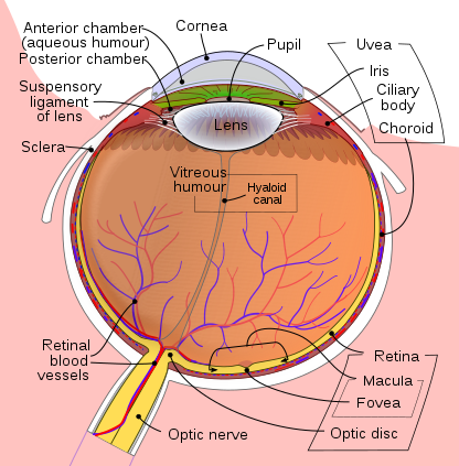
Figure 1. Eye. Rhcastilhos. And Jmarchn., CC BY-SA 3.0 <https://creativecommons.org/licenses/by-sa/3.0>, via Wikimedia Commons
The retina contains photoreceptor cells made of rods (sensitive to light) and cones (sensitive to color), bipolar cells, and ganglion cells (Figure 2). All these cells are neurons. The ganglion cells then form the optic nerve with their axons. Through the rods and cones, the photons generate electrical signals by phototransduction.
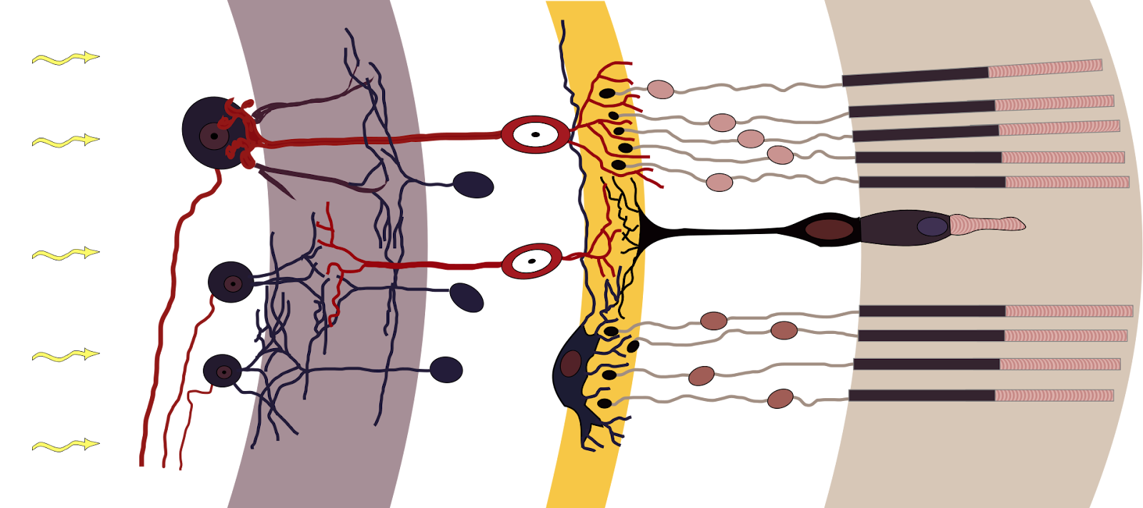
Figure 2. Retinal layers. By Fig_retine.png: Ramón y Cajalderivative work Fig retine bended.png: Anka Friedrich (talk)derivative work: vectorisation by chris 論 – Fig_retine.pngFig retine bended.png, CC BY-SA 3.0, https://commons.wikimedia.org/w/index.php?curid=7550631
The optic nerve then connects to the optic tract and to the Lateral geniculate nuclei (LNG, left and right) situated in the thalamus and then, in turn, connect to the Primary visual cortex through the optic radiations (Figure 3). The visual information is processed in the Primary visual cortex (also called the visual area V1).
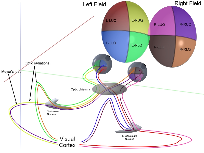
Figure 3. Optical cabling. Ratznium at en.wikipedia, CC BY-SA 3.0 <http://creativecommons.org/licenses/by-sa/3.0/>, via Wikimedia Commons
Hubel and Wiesel experiment
In 1958, Two scientists at Johns Hopkins University who later received the Nobel Prize in Medicine, David Hubel and Torsten Wiesel discovered that neurons in the striate cortex, part of the visual cortex, were activated by particular oriented lines and movements. They used kittens looking at a projector screen with tungsten microelectrodes inserted in the visual cortex connected to an oscilloscope to measure neuron activation. They initially investigated the neuron cell activation with black dots on a white slide till they accidentally showed the edge of the slide which triggered the neuron to fire. They found that field receptors on the neuron were being activated by specific oriented patterns (slit, dark bar, or edge) and movements. Some receptors were either excited or inhibited and have a particular geometry that matches the specific pattern they are reacting to. Neuron cells reacting to the same pattern are organized in vertical columns and neighboring cells are reacting to patterns of similar shape but slightly of different orientation.
Figure 4. Field receptors on a simple neuron cell are aligned with the pattern they react to
Convolutional Networks
Convolutional networks are inspired by the visual processing described in the previous section. Convolutional networks are particular cases of deep learning networks with layers of convolutions applied to images.
Convolution
Convolution is a mathematical operation that mixes two functions by multiplying their values by pairs. One version of convolution used in machine learning consists of multiplying pairs of values evaluated at the same point. This is called the cross-correlation.
One function works as the signal, the second function works as a filter. Figure 5 gives some examples of convolutional filters. The input signal is a 5×5 matrix with numerical values. It could be some color or light intensity. The input signal goes through the filter by multiplying each input cell by the corresponding filter cell in the same position. The input signal is then transformed into a filtered signal (also called the feature map). The output is calculated as the sum of all the values in the filtered signal.
The filters can be of different types. Each filter represents a different channel. Filter A at the top detects diagonal signals by filtering only values close to the main diagonal. Filter B detects horizontal signals and filter C detects signals on the secondary diagonal. If there is no overlap between the input signal and the filter, the final output value is zero. If the overlap is very large then the final output value is very large.
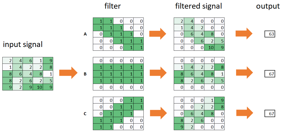
Figure 5. Examples of convolutional filters
The filters can amplify the input signal or even invert it (by using negative values). Like the neurons in the visual cortex, each filter is specialized in detecting special features.
An image is however larger and more complex than a 5×5 matrix. A solution is to use different filters and make them scan the image starting from left to right then top to bottom. This is illustrated in Figure 6 (with a 10×10 image and a 3×3 filter). The convolution operation starts with the top-left submatrix and continues to the subsequent matrices on the right by moving by one column (the stride which can be 1 or a higher value) till all the cells are covered and then towards the bottom by moving by one row (or more). The output ends up being an 8×8 matrix. To maintain the 10×10 size it is possible to add paddings of 0 values by adding extra rows and columns around the initial input image.
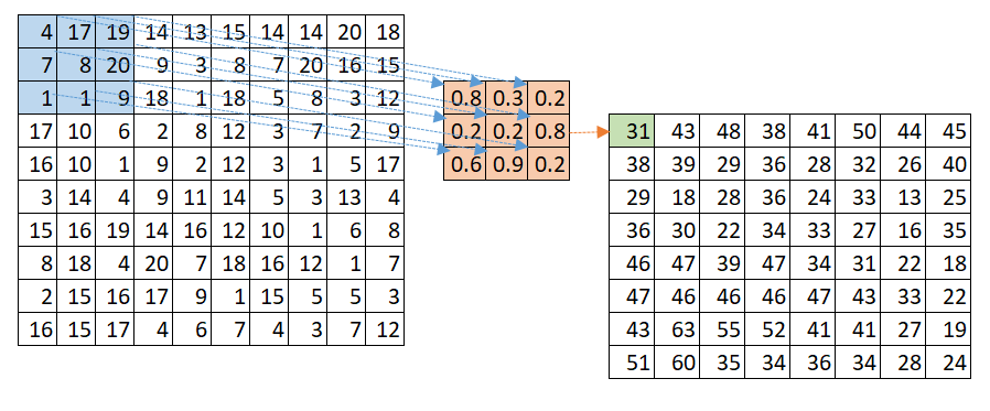
Figure 6. Convolutional Neural Network with a (3,3) Convolution
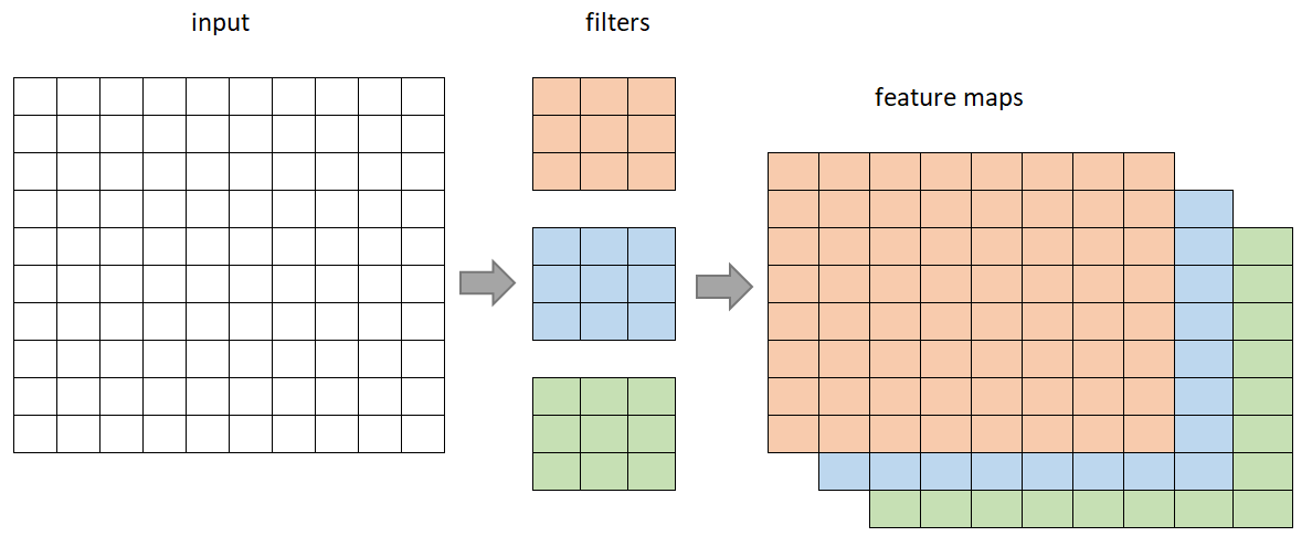
Figure 7. Convolutional Neural Network with 3 channels
Max pooling and average pooling
Besides convolution, another common operation is max pooling (Figure 8) and average pooling (Figure 9). With max pooling, the filter selects the maximum value of the matrix cells it is covering instead of multiplying the cells with some weights and summing the results. With average pooling, the filter calculates the average values of the matrix cells. Average pooling is a particular case of convolution where the weights in the filter have the same value and are normalized to sum up to one.
The pooling layers perform these pooling operations which aggregate the signals and downsize the image files (also called downsampling). Some information is lost during pooling operations. Some more recent techniques avoid pooling for that reason.

Figure 8. Convolutional Neural Network with Max Pooling
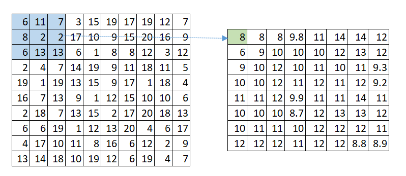
Figure 9. Convolutional Neural Network with Average Pooling
Translation equivariance
Convolutional networks have the property that they perform equally well at identifying and classifying an object if it moves horizontally or vertically in the image. The reason is that the same filters are also translated in the image. This is called translation equivariance. Convolutional networks are however not indifferent to rotation or inversion. They probably would be if filters were to rotate and be inverted. A solution is data augmentation. Images can be rotated and inverted and added to the training data.
Locality
Convolutional networks operate at the local level. They identify features in limited parts of the image as defined by the filter size and feed the features through several layers of neural networks.
Benchmarks
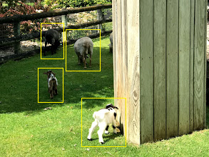
Figure 9. Image localization and identification
ImageNet
ImageNet is an image database created in 2009 by Professor Fei-Fei Li and her team as a benchmark for visual recognition and classification tasks. It contains over 14 million images from the internet annotated by humans around 20,000 categories called Synonym Sets (synsets). A higher-order category could be “fish” and be divided into hundreds of synsets of fish species that have hundreds of images of fish each. ImageNet is used for the ImageNet Large Scale Visual Recognition Challenge, started in 2010, in which researchers compete to detect and classify objects in images and videos. AlexNet (Krizhevsky et al., 2017) won the competition in 2012 using convolutional neural networks. The competition has been hosted by Kaggle since 2017. Its validation and test sets have 150,000 photographs and 1,000 categories. The training set is randomly sampled from these sets. Each photograph in the training and validation set has the coordinates of bounding boxes with the attached object category.
MNIST
MNIST is a dataset on handwritten digits that has been used by LeCun (1988) for visual recognition. It has 60,000 digits in the training set and 10,000 in the test set. Each digit occupies a 28×28 grid. 250 human writers, a mix of Census employees and high school students, created these digits in the training set and another 250 did the same for the test set.
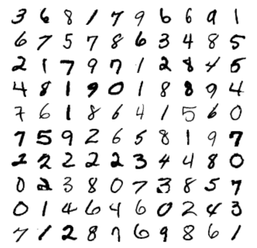
Figure 10. Examples of MNIST digits. Source LeCun et a;. 1998
Fashion MNIST
Fashion MNIST has the same structure as MNIST but is based on clothing articles from the company Zalando. Like MNIST, it has 60,000 images in the training set and 10,000 images in the test set. The size of each image is also 28×28. It also has ten categories ( 0: T-shirt/top, 1: Trouser, 2: Pullover, 3: Dress, 4: Coat, 5: Sandal, 6: Shirt, 7: Sneaker, 8: Bag, 9: Ankle boot). The difference is that the task is more difficult because the clothing articles have more variations than written digits.
Figure 11. Clothing articles from Fashion MNIST. Source: https://github.com/zalandoresearch/fashion-mnist/blob/master/doc/img/fashion-mnist-sprite.png
CIFAR-10 and CIFAR-100
CIFAR-10 is a dataset with 60,000 photos classified in 10 categories. CIFAR-100 is an extension of CIFAR-10 with 100 categories.
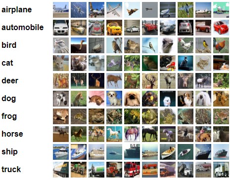
Figure 12. Photos from CIFAR-10. Source: https://www.cs.toronto.edu/~kriz/cifar.html
Convolutional Network Models
AlexNet
Building on convolution networks such as LeNet by (LeCun et al., 1989) (Figure 13), (Krizhevsky et al., 2012) proposed AlexNet in 2012 that won the ImageNet competition and put deep learning networks on the map for computer vision. They successfully classify 1.2 images into 1,000 classes with state-of-the-art results at the time.
AlexNet uses five convolutional layers, max-pooling layers, and three fully-connected layers (Figure 14) and ReLU activation functions. Images are of size 224×224 with three channels (RGB colors). To prevent overfitting, it performs data augmentation by extracting 224×224 patches and their inverses (horizontal reflections) from 256×256 images and by changing the RGB channel intensities. They also use dropout to reduce overfitting.
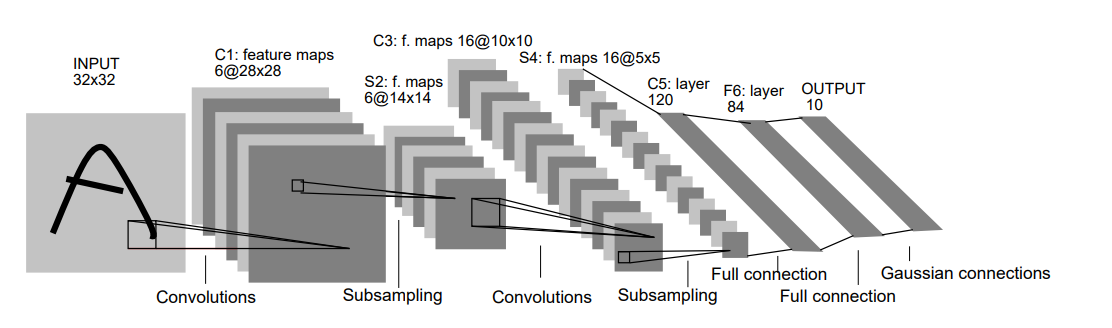
Figure 13. LeNet architecture
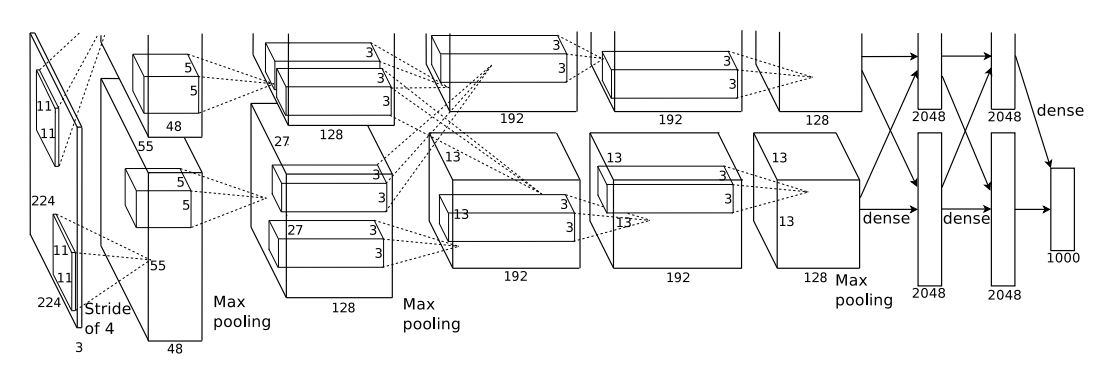
Figure 14. AlexNet architecture
GoogleNet
GoogleNet is based on the inception network as described in(Szegedy et al., 2014). A basic building block is the inception module. The inception modules were inspired by the Network in Network of (Lin et al., 2014). They allow a shift from sparse to dense representations using smaller filter-size convolutions (1×1, 3×3, 5×5), enhance the representativeness of the network and perform dimensionality reduction. The whole network will be built by stacking inceptions modules. These modules are stacked 22 times in GoogleNet.
In their inception module (Figure 15), a layer goes through three 1×1 convolutions and a 3×3 max pooling, then 3×3 convolutions, 5×5 convolutions and 1×1 convolutions. Outputs are then concatenated. The whole network is presented in Figure 16. GoogleNet achieves very good results in the ImageNet Large Scale Visual Recognition Challenge (ILSVRC) 2014 Classification (first) and Detection (second) Challenges.
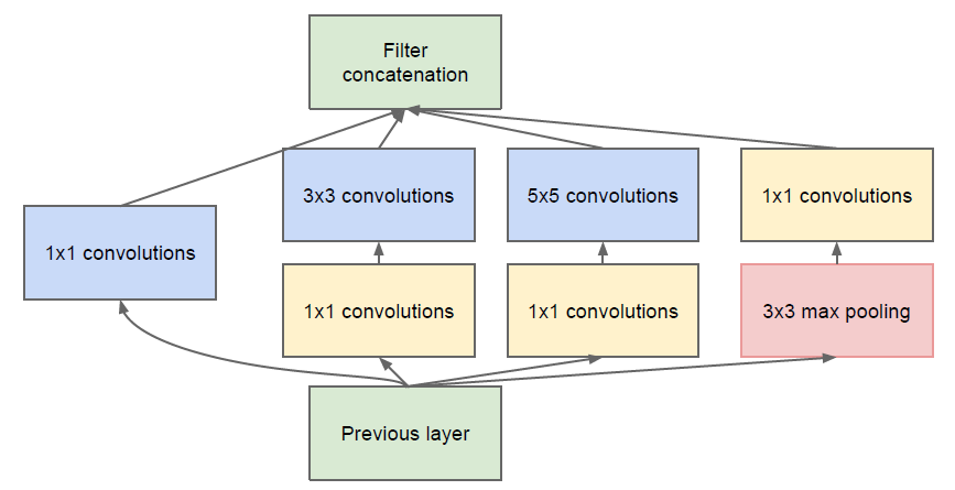
Figure 15. Inception module. Source: Szegedy et al., 2014
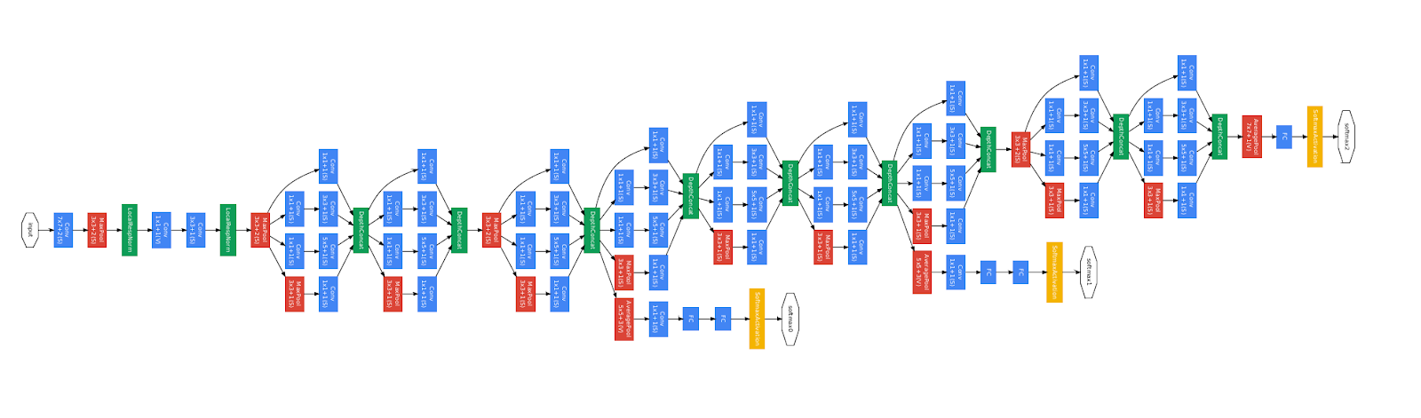
Figure 16. GoogleNet
VGG
VGGNet was introduced in (Simonyan and Zisserman, 2015) as an extension of standard convolutional networks such as LeNet and AlexNet with the difference that the network is deeper with 16-19 layers and with smaller (3×3) convolutional filters. They achieved 2nd and 1st place in the 2014 ImageNet Challenge in classification and localization. The increase in depth and the smaller receptive fields of the convolutions reduce the number of parameters compared to a standard convolutional network and work as a regularizer of the network. The configuration for VGG-16 (16 weight layers) combines stacked of two 3×3 convolutions with 64, 128, 256, 512, and 512 channels respectively, max-pooling layers and full and three fully connected layers of size 4096, 4096, and 1000 (for the 1000 classes). The activation function is ReLU. Figure 17 shows a truncated VGG-19 network.
ResNet
Residual networks (ResNet) introduced by (He et al., 2015b) are networks similar to VGG networks but with skip connections. These skip connections (Figure 17, the loops are the skip connections in the 34-Layer ResNet) connect inputs to outputs by adding the input values to the layer outputs coming from convolutional networks. Because the identity function is forced into the output at each step, the model focuses on fitting the residuals from the identity, a task that is easier to achieve as the authors have documented. Models can be very deep without encountering optimization problems or vanishing/exploding gradient issues. They evaluate their model on ImageNet and on CIFAR-10. Their ResNet model with 152 layers won the ILSVRC in 2015.
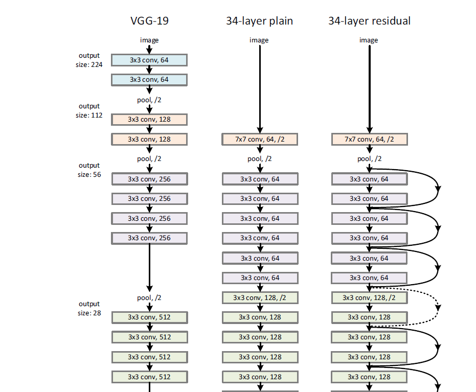
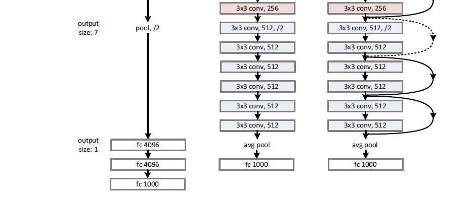
Figure 17. VGG Net vs 34-Layer plain and 34-Layer ResNet. Source: (He et al., 2015b)
References
Goodfellow, I., Bengio, Y., Courville, A., 2016. Deep Learning, Illustrated edition. ed. The MIT Press, Cambridge, Massachusetts.
He, K., Zhang, X., Ren, S., Sun, J., 2015a. Delving Deep into Rectifiers: Surpassing Human-Level Performance on ImageNet Classification. ArXiv150201852 Cs.
He, K., Zhang, X., Ren, S., Sun, J., 2015b. Deep Residual Learning for Image Recognition. ArXiv151203385 Cs.
Krizhevsky, A., Sutskever, I., Hinton, G.E., 2012. ImageNet Classification with Deep Convolutional Neural Networks. Adv. Neural Inf. Process. Syst. 25, 1097–1105.
LeCun, Y., Boser, B., Denker, J.S., Henderson, D., Howard, R.E., Hubbard, W., Jackel, L.D., 1989. Backpropagation applied to handwritten zip code recognition. Neural Comput. 1, 541–551. https://doi.org/10.1162/neco.1989.1.4.541
Lin, M., Chen, Q., Yan, S., 2014. Network In Network. ArXiv13124400 Cs.
Simonyan, K., Zisserman, A., 2015. Very Deep Convolutional Networks for Large-Scale Image Recognition. ArXiv14091556 Cs.
Srivastava, N., Hinton, G., Krizhevsky, A., Sutskever, I., Salakhutdinov, R., 2014. Dropout: A Simple Way to Prevent Neural Networks from Overfitting. J. Mach. Learn. Res. 15, 1929–1958.
Szegedy, C., Liu, W., Jia, Y., Sermanet, P., Reed, S., Anguelov, D., Erhan, D., Vanhoucke, V., Rabinovich, A., 2014. Going Deeper with Convolutions. ArXiv14094842 Cs.
Reproducibility, Reusability, and Robustness in Deep Reinforcement Learning
Mc Gill Professor Joelle Pineau has an insightful presentation on reproducibility in machine learning and especially in deep reinforcement learning. This is a general trend in science that some results sometimes cannot be fully reproduced. In deep reinforcement learning, there is a stochastic component to the results such as the present value of future rewards. She observes that results can vary for reasons that should not matter such as picking up a random seed (to generate random variables) and that the implementation of base cases by different researchers can yield different outcomes. Making the code and the data available for other researchers to reproduce paper results could alleviate some of these problems. She has introduced the Reproducibility Challenge that could be adopted by other scientific conferences.